Using factR
Fursham Hamid
2023-01-03
factR.RmdIntroduction
Many eukaryotic genes give rise to multiple RNA isoforms, increasing the protein-coding capacity of the genome and extending the range of post-transcriptional regulation possibilities. High-throughput sequencing is often used to deduce repertoires of transcripts expressed in specific biological samples by aligning the data to genomic sequences and assembling the alignments into transcript architectures. This typically outputs Gene Transfer Format (GTF) files describing newly identified transcripts as sets of exonic coordinates, but lacking the information about their coding sequences (CDSs; also known as ORFs) and possible biological functions.
To this end, we developed a package for functional annotation of custom-assembled transcriptomes in R (factR). factR predicts CDSs for novel RNA isoforms using a reference-guided process and then determines domain organisation of the protein products and possible susceptibility of transcripts to nonsense-mediated decay (NMD; a pathway destabilizing mRNAs with premature translation termination codons). factR also provides supporting tools for matching new transcripts to “official” gene IDs, visualizing transcript architectures and annotating alternatively spliced segments.
Getting started
Installing factR
To install factR, enter the following commands in your R environment:
if (!requireNamespace("BiocManager", quietly=TRUE))
    install.packages("BiocManager")
BiocManager::install("factR")
Materials needed
Custom-assembled transcriptome
factR requires a custom transcriptome file in the GTF format as an input, and we provide the following three sample custom transcriptome files that can be used to test factR tools:
-
bulk_merged_sample.gtf.gz assembled using the HISAT2-StringtTie2 pipeline (Pertea et al. 2016) from bulk RNA-seq data for mouse embryonic stem cells treated with the NMD inhibitor cycloheximide (CHX) or left untreated as a control.
- sc_merged_sample.gtf.gz assembled using the HISAT2-StringtTie2 pipeline from single-cell RNA-seq data for glutamatergic neurons, GABAergic neurons, astrocytes or endothelial cells from the mouse visual cortex (Tasic et al. 2018). A simplified version of this GTF containing the first 500 genes on chr15 is available as part of factR.
- lr_merged_sample.gtf.gz assembled using minimap2 (Li 2018) and StringtTie2 (Kovaka et al. 2019) from brain-specific long-read Oxford Nanopore RNA sequencing data (Sessegolo et al. 2019).
Method to download the above GTF files is described in the “Importing and inspecting GTF data” section below.
Users may alternatively prepare their own GTF files making sure that these contain both gene_id and transcript_id attributes.
Reference transcriptome
Several factR functions require reference transcriptome files (GTF or GFF3) as a guide. Such files can be accessed from within the R environment using e.g. the R package AnnotationHub or downloaded from an external database such as GENCODE or Ensembl. Both possibilities are described in the “Updating gene info” section below.
Genome
factR needs genomic DNA sequence to predict CDSs. Users may obtain genome files using e.g. BSgenome or AnnotationHub or download them from an external database such as GENCODE or Ensembl. We describe this in more detail in the “Constructing CDS information” section below.
Using factR
Load factR to the R environment as follows:
Importing and inspecting GTF data
factR handles transcriptome information in the form of GenomicRanges objects containing genomic interval data and relevant metadata. To create such an object from a GTF file, we use the importGTF function:
gtf <- system.file("extdata", "sc_merged_sample.gtf.gz", package = "factR")
custom.gtf <- importGTF(gtf)
The imported GTF file is stored as a GenomicRanges object.
class(custom.gtf)
#> [1] "GRanges"
#> attr(,"package")
#> [1] "GenomicRanges"
Contents of the object can be examined using head:
head(custom.gtf)
#> GRanges object with 6 ranges and 9 metadata columns:
#>       seqnames          ranges strand |    source       type     score
#>          <Rle>       <IRanges>  <Rle> |  <factor>   <factor> <numeric>
#>   [1]    chr15 3180731-3180944      * | StringTie transcript      1000
#>   [2]    chr15 3180731-3180944      * | StringTie exon            1000
#>   [3]    chr15 3217391-3219698      - | StringTie transcript      1000
#>   [4]    chr15 3217391-3219698      - | StringTie exon            1000
#>   [5]    chr15 3268547-3277274      + | StringTie transcript      1000
#>   [6]    chr15 3268547-3268768      + | StringTie exon            1000
#>           phase     gene_id        transcript_id exon_number   gene_name
#>       <integer> <character>          <character> <character> <character>
#>   [1]      <NA> MSTRG.14523        MSTRG.14523.1        <NA>        <NA>
#>   [2]      <NA> MSTRG.14523        MSTRG.14523.1           1        <NA>
#>   [3]      <NA> MSTRG.14524 ENSMUST00000227053.1        <NA>      Gm7962
#>   [4]      <NA> MSTRG.14524 ENSMUST00000227053.1           1      Gm7962
#>   [5]      <NA> MSTRG.14525 ENSMUST00000160787.8        <NA>     Selenop
#>   [6]      <NA> MSTRG.14525 ENSMUST00000160787.8           1     Selenop
#>                 ref_gene_id
#>                 <character>
#>   [1]                  <NA>
#>   [2]                  <NA>
#>   [3]  ENSMUSG00000114999.1
#>   [4]  ENSMUSG00000114999.1
#>   [5] ENSMUSG00000064373.12
#>   [6] ENSMUSG00000064373.12
#>   -------
#>   seqinfo: 1 sequence from an unspecified genome; no seqlengths
In addition to genomic coordinates (seqnames and ranges), a typical GTF file contains metadata describing the feature type (e.g. transcript or exon), transcript IDs and some information on their parental genes.
Use the following command to calculate the total number of transcripts in the input transcriptome:
Note that none of the transcripts in the custom.gtf object contain CDS information:
Plotting transcript structures
Users may visualize specific sets of transcripts using viewTranscripts. For example, the following will plot transcripts from the Zfr gene encoding a conserved zinc finger-containing RNA-binding protein with known neuronal functions :
viewTranscripts(custom.gtf, "Zfr") 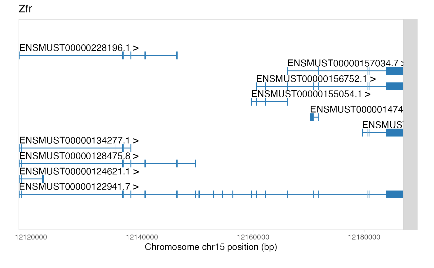
StringTie2, a popular transcript assembler used to generate our custom GTF, typically assigns arbitrary names to newly identified transcripts (e.g. “MSTRG.x.y”) and uses the same prefix for their gene IDs (e.g. “MSTRG.x”). Incidentally, this is why the output above contains 10 previously known Zfr transcripts but lacks any novel entries.
Updating gene info
factR can update gene metadata in custom transcriptome objects using a reference annotation as guide. Below, we describe two alternative ways to obtain mouse reference transcriptome data from GENCODE.
- Using AnnotationHub package
# query database for mouse gencode basic annotation
library(AnnotationHub)
ah <- AnnotationHub()
#> snapshotDate(): 2022-10-31
query(ah, c('Mus musculus', 'gencode', 'gff'))
#> AnnotationHub with 9 records
#> # snapshotDate(): 2022-10-31
#> # $dataprovider: Gencode
#> # $species: Mus musculus
#> # $rdataclass: GRanges
#> # additional mcols(): taxonomyid, genome, description,
#> #   coordinate_1_based, maintainer, rdatadateadded, preparerclass, tags,
#> #   rdatapath, sourceurl, sourcetype
#> # retrieve records with, e.g., 'object[["AH49545"]]'
#>
#>             title
#>   AH49545 | gencode.vM6.2wayconspseudos.gff3.gz
#>   AH49546 | gencode.vM6.annotation.gff3.gz
#>   AH49547 | gencode.vM6.basic.annotation.gff3.gz
#>   AH49548 | gencode.vM6.chr_patch_hapl_scaff.annotation.gff3.gz
#>   AH49549 | gencode.vM6.chr_patch_hapl_scaff.basic.annotation.gff3.gz
#>   AH49550 | gencode.vM6.long_noncoding_RNAs.gff3.gz
#>   AH49551 | gencode.vM6.polyAs.gff3.gz
#>   AH49552 | gencode.vM6.primary_assembly.annotation.gff3.gz
#>   AH49553 | gencode.vM6.tRNAs.gff3.gz

# Download full annotation
ref.gtf <- ah[['AH49546']]
#> downloading 1 resources
#> retrieving 1 resource
#> loading from cache- Downloading from a GENCODE database (ref.gtf generated from this method will be used for the remaining of the workflow)
tmp <- tempfile()
download.file("ftp://ftp.ebi.ac.uk/pub/databases/gencode/Gencode_mouse/release_M25/gencode.vM25.annotation.gtf.gz",
              destfile = tmp)
ref.gtf <- importGTF(tmp)
When choosing a reference, users should consider using one with the same chromosome naming style (e.g. “chr1” or “1”). Alternatively, the styles can be matched using the matchChromosomes function (see help(matchChromosomes) for more detail).
Once the ref.gtf object is ready, novel transcripts in custom.gtf can be assigned to “official” gene IDs, whenever possible, using matchGeneInfo. By default, this function matches the query (custom.gtf) to the reference (ref.gtf) by finding overlapping coordinates:
# matching gene metadata
custom_matched_1.gtf <- matchGeneInfo(custom.gtf, ref.gtf)
#>     Number of mismatched gene_ids found: 500
#>     ---> Attempting to match gene_ids by finding overlapping coordinates...
#>     ---> 386 gene_id matched
#>     Total gene_ids corrected: 386
#>     Remaining number of mismatched gene_ids: 114
To tune the performance of matchGeneInfo, we provide additional arguments specifying the name of columns containing “primary” and potentially “secondary” gene IDs from the query (custom.gtf). For further information, see help(matchGeneInfo).
# matching gene metadata
custom_matched_2.gtf <- matchGeneInfo(custom.gtf, ref.gtf,
                            primary_gene_id = "gene_id",
                            secondary_gene_id = "ref_gene_id")
#>     Number of mismatched gene_ids found: 500
#>     -> Attempting to correct gene ids by replacing gene_id with ref_gene_id...
#>     -> 212 gene_ids matched
#>     --> Attempting to match ensembl gene_ids...
#>     --> All ensembl gene ids have been matched
#>     ---> Attempting to match gene_ids by finding overlapping coordinates...
#>     ---> 174 gene_id matched
#>     Total gene_ids corrected: 386
#>     Remaining number of mismatched gene_ids: 114
Note that custom.gtf updated by matchGeneInfo now contains 10 known and 7 newly Zfr assembled transcripts:
viewTranscripts(custom_matched_2.gtf, "Zfr") 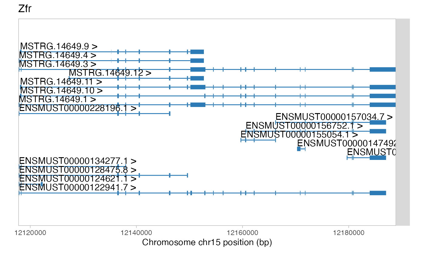
Shortlisting novel transcripts
As seen in the above example, custom transcriptomes typically combine both new and previously annotated transcripts. To select only newly predicted transcripts, run the following:
custom_new.gtf <- subsetNewTranscripts(custom_matched_2.gtf, ref.gtf)
#> Removing transcripts with exact exon coordinates

viewTranscripts(custom_new.gtf,"Zfr") 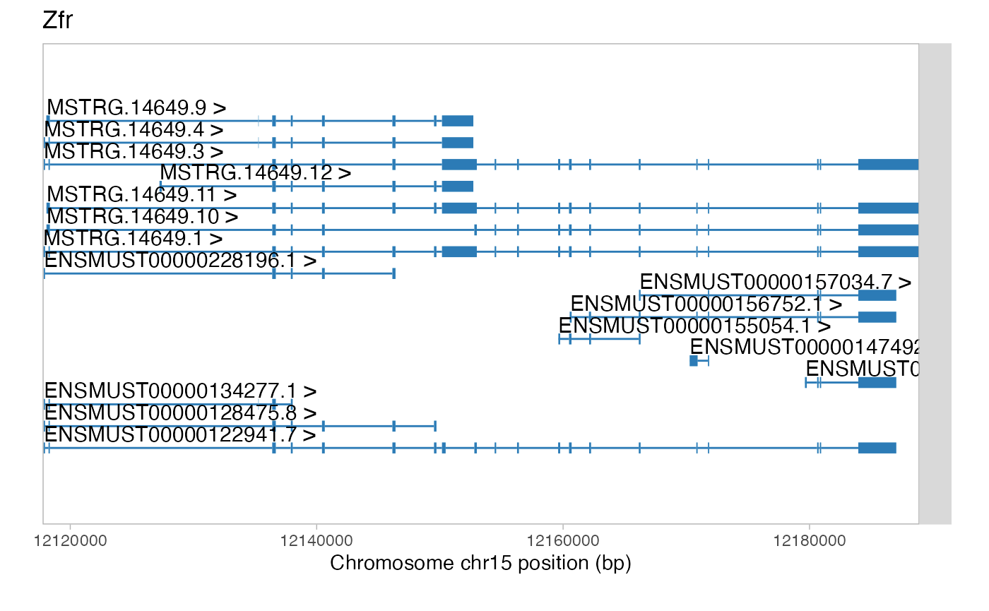
This will subset custom.gtf transcripts with distinct exonic coordinates compared to ref.gtf and will store these transcripts in the custom_new.gtf object. Some custom-built transcripts may differ from their reference counterparts by having different start or/and end coordinates, with otherwise similar exon-intron structure. To shortlist novel transcripts with distinct intronic coordinates only, simply set the “refine.by” argument to “intron”:
custom_new.gtf <- subsetNewTranscripts(custom_matched_2.gtf, ref.gtf, refine.by = "intron")
#> Removing transcripts with exact exon coordinates
#> Removing transcripts with exact intron coordinates

viewTranscripts(custom_new.gtf, "Zfr") 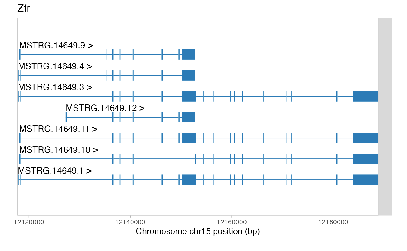
We will use the custom_new.gtf object in the rest of the workflow.
Constructing CDS information
Functional annotation of newly assembled transcripts in factR begins by deducing their protein-coding sequences (CDSs). To search for putative CDSs, factR requires a genome sequence file, which can be obtained using R packages or downloaded from online databases (e.g. UCSC, GENCODE or Ensembl). Three alternative ways to retrieve mouse genomic sequence are described below.
- Using BSgenome (Mmusculus generated from this method will be used for the remaining of the workflow) This package supports most sequenced genomes. Mouse mm10 sequence can be downloaded as follows:
if (!requireNamespace("BiocManager", quietly = TRUE))
    install.packages("BiocManager")

BiocManager::install("BSgenome.Mmusculus.UCSC.mm10")
and loaded into R environment:
library(BSgenome.Mmusculus.UCSC.mm10)
Mmusculus <- BSgenome.Mmusculus.UCSC.mm10- Using AnnotationHub
library(AnnotationHub)
ah <- AnnotationHub()
#> snapshotDate(): 2022-10-31
query(ah, c("mm10","2bit"))
#> AnnotationHub with 1 record
#> # snapshotDate(): 2022-10-31
#> # names(): AH14005
#> # $dataprovider: UCSC
#> # $species: Mus musculus
#> # $rdataclass: TwoBitFile
#> # $rdatadateadded: 2014-12-15
#> # $title: mm10.2bit
#> # $description: UCSC 2 bit file for mm10
#> # $taxonomyid: 10090
#> # $genome: mm10
#> # $sourcetype: TwoBit
#> # $sourceurl: http://hgdownload.cse.ucsc.edu/goldenpath/mm10/bigZips/mm10.2bit
#> # $sourcesize: NA
#> # $tags: c("2bit", "UCSC", "genome")
#> # retrieve record with 'object[["AH14005"]]'
# Retrieve mouse genome
Mmusculus <- ah[['AH14005']] - Downloading from a database (e.g. GENCODE)
tmp <- tempfile()
download.file("ftp://ftp.ebi.ac.uk/pub/databases/gencode/Gencode_mouse/release_M25/GRCm38.primary_assembly.genome.fa.gz",
              tmp)
Mmusculus <- importFASTA(paste0(tmp, "/GRCm38.primary_assembly.genome.fa.gz"))
Once the genome sequence object is ready, factR can predict CDSs using its buildCDS() function and reference transcriptome data as a guide. buildCDS() first generates a database of previously annotated ATGs and uses this information to search for a potential translation start sites in query transcripts. buildCDS() then deduces the CDS and appends its coordinates to the custom transcriptome object. Let’s run this function for our novel transcripts:
custom_new_CDS.gtf <- buildCDS(custom_new.gtf, ref.gtf, Mmusculus)
#>     Searching for reference mRNAs in query
#>     No reference mRNAs found
#>     Building database of annotated ATG codons
#>     Selecting best ATG start codon for remaining transcripts and determining open-reading frame
#>     114 new CDSs constructed
#>
#>     Summary: Out of 380 transcripts in `custom_new.gtf`,
#>     114 transcript CDSs were built
Note that the novel Zfr transcripts have been updated with information about likely CDSs (dark blue) and untranslated regions (light blue) :
viewTranscripts(custom_new_CDS.gtf, "Zfr") 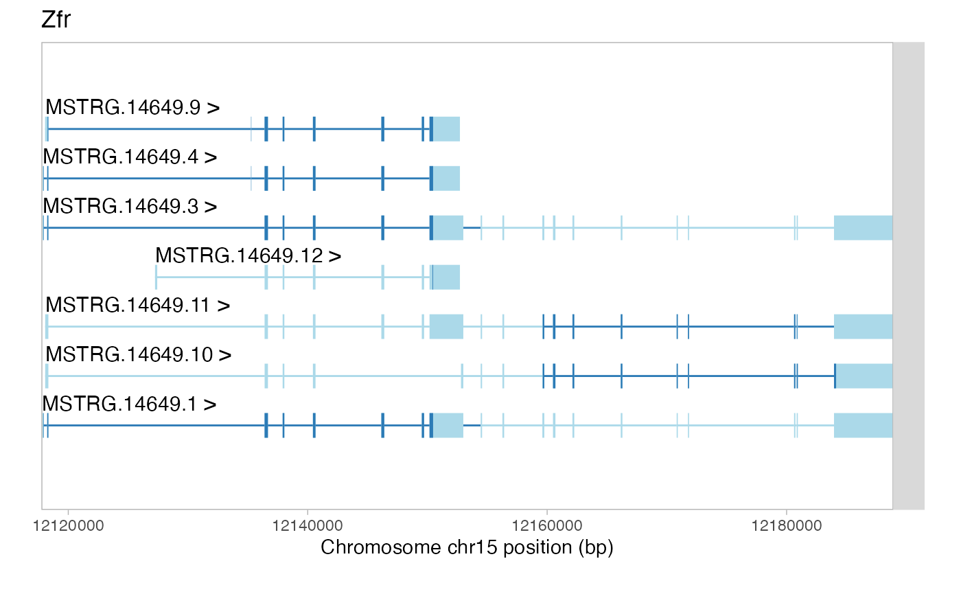
We can display exonic regions and CDSs more clearly (at the expense of loosing their bona fide genomic coordinates) by setting rescale_intron argument to TRUE.
viewTranscripts(custom_new_CDS.gtf, "Zfr", rescale_introns = TRUE) 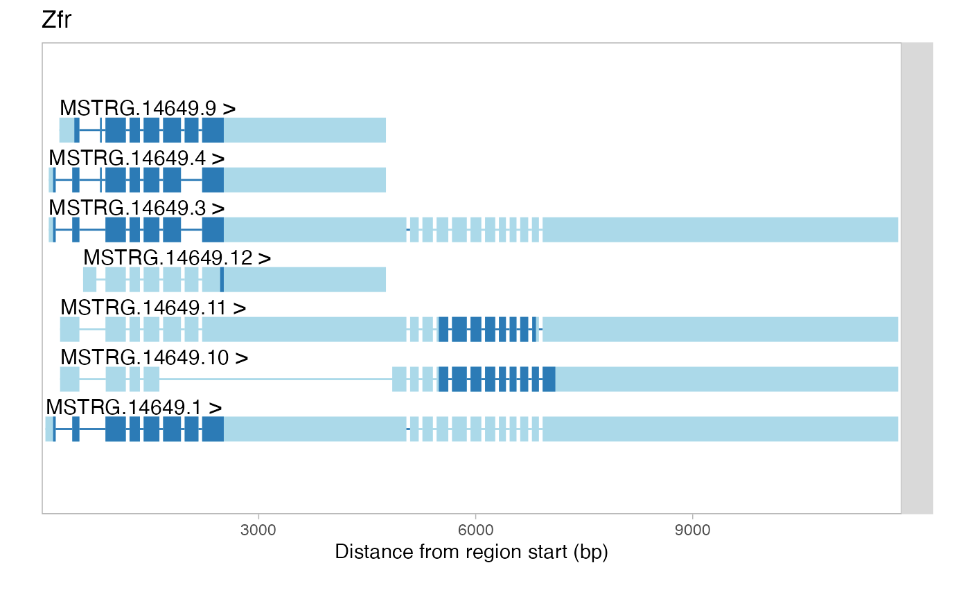
For comparison, here is the CDS situation in the reference Zfr transcripts:
viewTranscripts(ref.gtf, "Zfr", rescale_introns = TRUE) 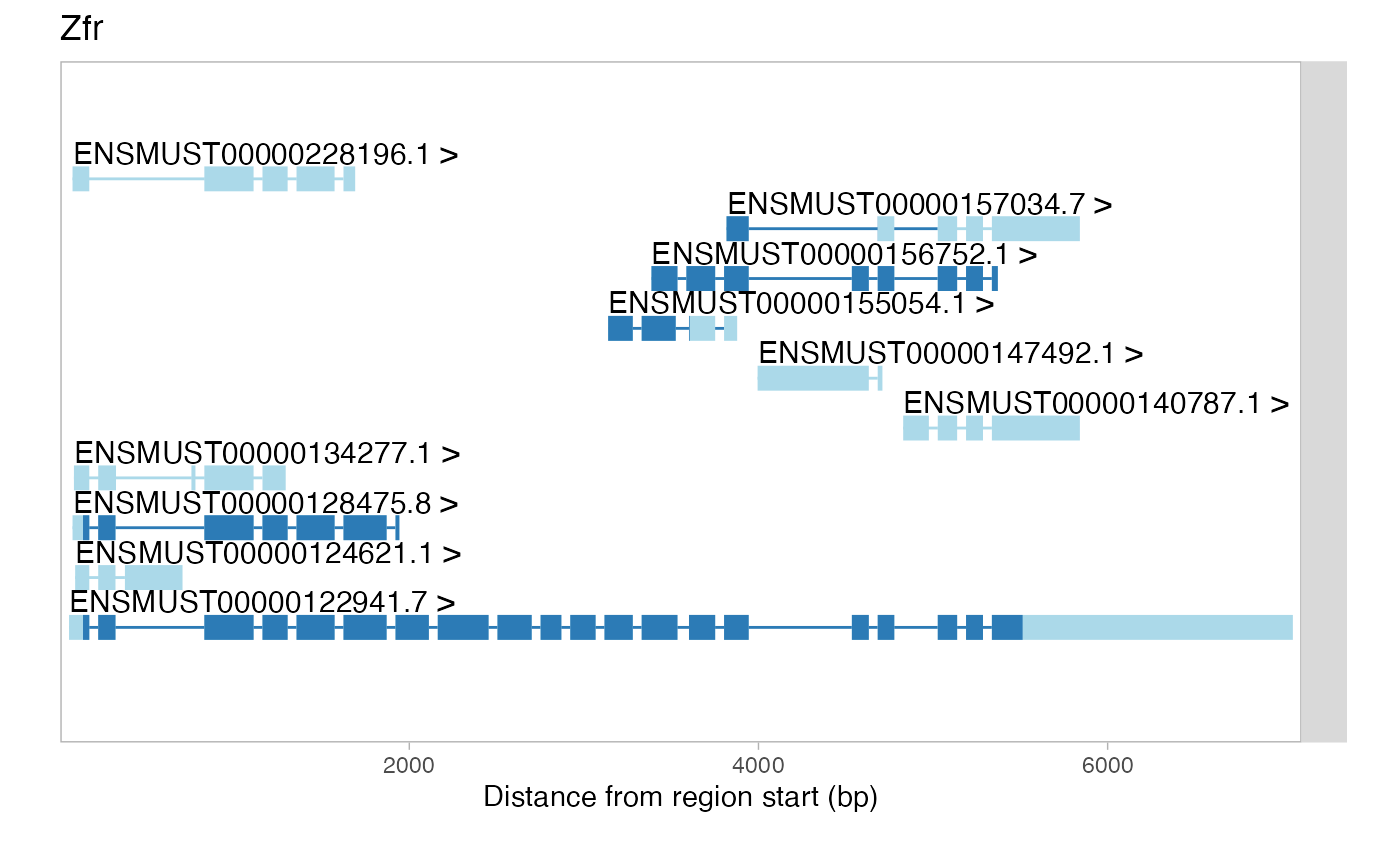
Predicting NMD
To explore possible susceptibility of newly identified mRNA isoforms to NMD, we use the predictNMD function:
NMDprediction.out <- predictNMD(custom_new_CDS.gtf)
#> Predicting NMD sensitivities for 114 mRNAs
head(NMDprediction.out)
#> # A tibble: 6 × 6
#> transcript stop_to_lastEJ num_of_downEJs 3'UTR_leng…¹ is_NMD PTC_c…²
#> <chr> <dbl> <int> <dbl> <lgl> <chr>
#> 1 ENSMUST00000100790.3 222 3 2895 TRUE chr15:…
#> 2 ENSMUST00000228827.1 NA 0 1672 FALSE NA
#> 3 MSTRG.14527.7 -131 0 2244 FALSE NA
#> 4 MSTRG.14531.1 1937 9 4141 TRUE chr15:…
#> 5 MSTRG.14531.5 872 3 5317 TRUE chr15:…
#> 6 MSTRG.14533.2 1073 1 2541 TRUE chr15:…
#> # … with abbreviated variable names ¹`3'UTR_length`, ²PTC_coordpredictNMD outputs a data frame containing information on features that may promote NMD and predicts NMD sensitivity for each CDS-containing transcript based on the distance between the stop codon and the last exon-exon junction.
To identify putative NMD targets for specific genes (e.g. Zfr), run the following:
NMDprediction.Zfr <- predictNMD(custom_new_CDS.gtf, gene_name == "Zfr")
#>  Predicting NMD sensitivities for 7 mRNAs

head(NMDprediction.Zfr)
#> # A tibble: 6 × 6
#>   transcript     stop_to_lastEJ num_of_downEJs `3'UTR_length` is_NMD PTC_coord
#>   <chr>                   <dbl>          <int>          <dbl> <lgl>  <chr>
#> 1 MSTRG.14649.1            3857             11           8774 TRUE   chr15:1215…
#> 2 MSTRG.14649.10           -177              0           4740 FALSE  NA
#> 3 MSTRG.14649.11             41              1           4958 FALSE  NA
#> 4 MSTRG.14649.12           -300              0           2242 FALSE  NA
#> 5 MSTRG.14649.3            3857             11           8774 TRUE   chr15:1215…
#> 6 MSTRG.14649.4            -300              0           2242 FALSE  NA
Predicting protein domains
factR can also inspect domain structure of protein products encoded by newly identified mRNA isoforms using its predictDomains() function. This requires connection to the online PFAM database and may require a substantial amount of time and stable internet connection to query multiple transcripts simultaneously. To quickly explore functionality of the predictDomains() tool, users may prefer to begin with a relatively small subset of transcripts. For example, the following will predict domain structure for all transcripts of the Zfr gene:
predictDomains(custom_new_CDS.gtf, Mmusculus, gene_name == "Zfr", progress_bar = FALSE)
#> Checking CDSs and translating protein sequences
#> Predicting domain families for 7 proteins
#> # A tibble: 6 × 5
#>   transcript    description                  eval     begin   end
#>   <chr>         <chr>                        <chr>    <dbl> <dbl>
#> 1 MSTRG.14649.1 beta-beta-alpha zinc fingers 1.54e-20   303   364
#> 2 MSTRG.14649.1 beta-beta-alpha zinc fingers 1.54e-20   371   414
#> 3 MSTRG.14649.3 beta-beta-alpha zinc fingers 1.54e-20   303   350
#> 4 MSTRG.14649.4 beta-beta-alpha zinc fingers 1.54e-20   311   358
#> 5 MSTRG.14649.9 beta-beta-alpha zinc fingers 1.54e-20   289   350
#> 6 MSTRG.14649.9 beta-beta-alpha zinc fingers 1.54e-20   357   400
The domain architectures for the set of query proteins can be additionally plotted by switching the argument “plot” to TRUE:
domains.Zfr <- predictDomains(custom_new_CDS.gtf, Mmusculus, gene_name == "Zfr", plot = TRUE, progress_bar = FALSE) If you want to predict domains for all new transcripts and do not mind waiting for some time depending on the connection speed and the PFAM server load, run the following:
domains.out <- predictDomains(custom_new_CDS.gtf, Mmusculus, progress_bar = FALSE) Export output objects
Annotated custom_new_CDS.gtf object can be exported to a GTF file as follows:
library(rtracklayer)
export(custom_new_CDS.gtf, "Custom_new.gtf", format = "GTF")
Finally, to export NMDprediction.out and domains.out data frames as tab-delimited text files, run the following:
write.table(NMDprediction.out, "Custom_new_NMD.txt", sep = "\t", row.names = FALSE, quote = FALSE)
write.table(domains.out, "Custom_new_domains.txt", sep = "\t", row.names = FALSE, quote = FALSE) Session Information
This workflow was conducted on:
sessionInfo()
#> R version 4.2.2 (2022-10-31)
#> Platform: x86_64-apple-darwin17.0 (64-bit)
#> Running under: macOS Big Sur ... 10.16
#>
#> Matrix products: default
#> BLAS:   /Library/Frameworks/R.framework/Versions/4.2/Resources/lib/libRblas.0.dylib
#> LAPACK: /Library/Frameworks/R.framework/Versions/4.2/Resources/lib/libRlapack.dylib
#>
#> locale:
#> [1] en_US.UTF-8/en_US.UTF-8/en_US.UTF-8/C/en_US.UTF-8/en_US.UTF-8
#>
#> attached base packages:
#> [1] stats4    stats     graphics  grDevices utils     datasets  methods
#> [8] base
#>
#> other attached packages:
#>  [1] forcats_0.5.2                      stringr_1.5.0
#>  [3] dplyr_1.0.10                       purrr_1.0.0
#>  [5] readr_2.1.3                        tidyr_1.2.1
#>  [7] tibble_3.1.8                       ggplot2_3.4.0
#>  [9] tidyverse_1.3.2                    GenomicFeatures_1.50.3
#> [11] AnnotationDbi_1.60.0               Biobase_2.58.0
#> [13] BSgenome.Mmusculus.UCSC.mm10_1.4.3 BSgenome_1.66.1
#> [15] rtracklayer_1.58.0                 GenomicRanges_1.50.2
#> [17] Biostrings_2.66.0                  GenomeInfoDb_1.34.4
#> [19] XVector_0.38.0                     IRanges_2.32.0
#> [21] S4Vectors_0.36.1                   AnnotationHub_3.6.0
#> [23] BiocFileCache_2.6.0                dbplyr_2.2.1
#> [25] BiocGenerics_0.44.0                factR_1.1.1
#>
#> loaded via a namespace (and not attached):
#>   [1] readxl_1.4.1                  backports_1.4.1
#>   [3] systemfonts_1.0.4             BiocParallel_1.32.5
#>   [5] digest_0.6.31                 htmltools_0.5.4
#>   [7] fansi_1.0.3                   magrittr_2.0.3
#>   [9] memoise_2.0.1                 googlesheets4_1.0.1
#>  [11] tzdb_0.3.0                    modelr_0.1.10
#>  [13] matrixStats_0.63.0            timechange_0.1.1
#>  [15] pkgdown_2.0.7                 prettyunits_1.1.1
#>  [17] colorspace_2.0-3              blob_1.2.3
#>  [19] rvest_1.0.3                   rappdirs_0.3.3
#>  [21] textshaping_0.3.6             haven_2.5.1
#>  [23] xfun_0.36                     crayon_1.5.2
#>  [25] RCurl_1.98-1.9                jsonlite_1.8.4
#>  [27] glue_1.6.2                    gtable_0.3.1
#>  [29] gargle_1.2.1                  zlibbioc_1.44.0
#>  [31] DelayedArray_0.24.0           scales_1.2.1
#>  [33] DBI_1.1.3                     Rcpp_1.0.9
#>  [35] xtable_1.8-4                  progress_1.2.2
#>  [37] bit_4.0.5                     httr_1.4.4
#>  [39] ellipsis_0.3.2                pkgconfig_2.0.3
#>  [41] XML_3.99-0.13                 farver_2.1.1
#>  [43] sass_0.4.4                    utf8_1.2.2
#>  [45] tidyselect_1.2.0              labeling_0.4.2
#>  [47] rlang_1.0.6                   later_1.3.0
#>  [49] munsell_0.5.0                 BiocVersion_3.16.0
#>  [51] cellranger_1.1.0              tools_4.2.2
#>  [53] cachem_1.0.6                  cli_3.5.0
#>  [55] generics_0.1.3                RSQLite_2.2.20
#>  [57] broom_1.0.2                   evaluate_0.19
#>  [59] fastmap_1.1.0                 yaml_2.3.6
#>  [61] ragg_1.2.4                    knitr_1.41
#>  [63] bit64_4.0.5                   fs_1.5.2
#>  [65] KEGGREST_1.38.0               pbapply_1.6-0
#>  [67] mime_0.12                     xml2_1.3.3
#>  [69] biomaRt_2.54.0                compiler_4.2.2
#>  [71] filelock_1.0.2                curl_4.3.3
#>  [73] png_0.1-8                     interactiveDisplayBase_1.36.0
#>  [75] reprex_2.0.2                  bslib_0.4.2
#>  [77] stringi_1.7.8                 highr_0.10
#>  [79] desc_1.4.2                    lattice_0.20-45
#>  [81] Matrix_1.5-1                  vctrs_0.5.1
#>  [83] pillar_1.8.1                  lifecycle_1.0.3
#>  [85] BiocManager_1.30.19           jquerylib_0.1.4
#>  [87] data.table_1.14.6             bitops_1.0-7
#>  [89] wiggleplotr_1.22.0            httpuv_1.6.7
#>  [91] patchwork_1.1.2               R6_2.5.1
#>  [93] BiocIO_1.8.0                  promises_1.2.0.1
#>  [95] codetools_0.2-18              assertthat_0.2.1
#>  [97] SummarizedExperiment_1.28.0   rprojroot_2.0.3
#>  [99] rjson_0.2.21                  withr_2.5.0
#>  [ reached getOption("max.print") -- omitted 12 entries ]
References
Kovaka, Sam, Aleksey V. Zimin, Geo M. Pertea, Roham Razaghi, Steven L. Salzberg, and Mihaela Pertea. 2019. “Transcriptome Assembly from Long-Read Rna-Seq Alignments with Stringtie2.” Genome Biology 20 (1): 278. https://doi.org/10.1186/s13059-019-1910-1.
Li, Heng. 2018. “Minimap2: Pairwise Alignment for Nucleotide Sequences.” Bioinformatics 34 (18): 3094–3100. https://doi.org/10.1093/bioinformatics/bty191.
Pertea, Mihaela, Daehwan Kim, Geo M. Pertea, Jeffrey T. Leek, and Steven L. Salzberg. 2016. “Transcript-Level Expression Analysis of Rna-Seq Experiments with Hisat, Stringtie and Ballgown.” Nature Protocols 11 (9): 1650–67. https://doi.org/10.1038/nprot.2016.095.
Sessegolo, Camille, Corinne Cruaud, Corinne Da Silva, Audric Cologne, Marion Dubarry, Thomas Derrien, Vincent Lacroix, and Jean-Marc Aury. 2019. “Transcriptome Profiling of Mouse Samples Using Nanopore Sequencing of cDNA and Rna Molecules.” Scientific Reports 9 (1): 14908. https://doi.org/10.1038/s41598-019-51470-9.
Tasic, Bosiljka, Zizhen Yao, Lucas T. Graybuck, Kimberly A. Smith, Thuc Nghi Nguyen, Darren Bertagnolli, Jeff Goldy, et al. 2018. “Shared and Distinct Transcriptomic Cell Types Across Neocortical Areas.” Nature 563 (7729): 72–78. https://doi.org/10.1038/s41586-018-0654-5.